Probability Mass Functions: The Unsung Heroes Behind Every “Generate” Button You’ve Ever Clicked

“If probability is the language of uncertainty, a PMF is its grammar: crisp, discrete, and occasionally punch‑line worthy.”

Picture this: You open your favorite generative‑AI app, type “Write me a haiku about mangoes,” and in less time than it takes to blink, a tiny digital poet complies. What sorcery decides which 17 syllables appear? Beneath the glittery UI sits a humble probability mass function (PMF), a mathematical table of possibilities assigning each next‑word (or pixel, or musical note) a neatly wrapped probability. In other words, your chatbot is basically rolling a 50‑billion‑sided die with weighted faces. (The house rule is no snake eyes on “mango.”)

In our data-driven world, especially in the buzzing domain of Artificial Intelligence, we’re constantly dealing with scenarios that have a specific, countable number of outcomes. Will a user click this ad (yes/no)? How many defective items are in this batch? What rating (1 to 5 stars) will a customer give? To make sense of this discrete world, we need a special kind of map – a map that tells us the exact probability of each specific outcome. Enter, stage left, the unsung hero: the Probability Mass Function (PMF).

By the end of this post you’ll not only know how that die is forged, you’ll forge a few of your own in Python—because nothing says “power user” like summoning your own PMFs at will. Ready? Let’s roll.

Prefer watching, here is the video version, slightly condensed of this blog post:

Hold Up, What Do You Mean “Discrete”? Let’s Talk Random Variables!

Before we get intimate with PMFs, we need to quickly high-five its best friend: the Discrete Random Variable. Imagine a random variable as a placeholder for a number that comes out of some random process. Now, if this number can only take on specific, separate, countable values (often integers), then bingo, it’s discrete.

Think of it like this:

Discrete: The number of samosas you can devour (you can’t eat 2.7 samosas, unless things get messy). The number of sixes Virat Kohli hits in an over (0, 1, 2,… up to 6). The number of new followers you got today.
Not Discrete (Continuous): The exact height of a person (could be 175.2345… cm). The precise time it takes for your code to run. These can take any value within a range.

PMFs are the rockstars for the discrete stuff. For the continuous gang, their cousin, the PDF (Probability Density Function), takes the stage – but that’s a story for another blog post!

Why Bother With PMFs Anyway?

A PMF answers the question “What is the probability that a discrete random variable takes value x?” It’s foundational in:

Machine learning models (classification probabilities).
Natural‑language processing (next‑token distributions).
Risk analysis (yes/no events).
Your daily life (deciding whether you’ll get a parking spot—spoiler: the odds are never in your favor).

In simple terms, a Probability Mass Function (PMF), denoted as $P(X=x)$ or $p_X(x)$, tells you the probability that a discrete random variable $X$ will be exactly equal to some specific value $x$.

It’s like asking, “What’s the probability I roll exactly a 4 on this die?” or “What’s the probability exactly 3 out of 5 users will click on the ‘buy now’ button?” The PMF hands you the answer on a silver platter (with probabilities, not actual silver, unfortunately).

In Generative AI, PMFs sit at the final layer: the softmax over possible tokens. Alter them—clip the tail (Top‑k), shave the body (nucleus sampling), or spice them up with temperature—and your model’s “personality” flips faster than a barista who just ran out of espresso beans.

The PMF’s Golden Rules (Its Properties):

Every self-respecting PMF lives by two sacred rules, or else it’s just a pretender:

Rule #1: No Negative Vibes Allowed! $(P(X=x)≥0)$ The probability of any specific outcome must be greater than or equal to zero. You can’t have a -10% chance of rolling a 3. That’s just silly talk. Probabilities are optimists; they’re always zero or positive.
Rule #2: It All Adds Up! If you take all the possible distinct outcomes for your discrete random variable and sum up their individual probabilities, you must get 1 (or 100%). $$\sum\limits_{x}P(X=x)=1$$ This makes perfect sense, right? One of the possible outcomes has to happen. The universe isn’t going to just shrug and say, “None of the above today, try again tomorrow.”

Think of it like a pizza. Each slice (outcome) has a certain size (probability). All the slices together make one whole pizza (total probability of 1). If they don’t, someone’s been sneakily eating the evidence, or it’s not a valid PMF! Here are few more real world glimpses on where our friend PMF comes handy:

Coin toss (Bernoulli): Heads vs. tails.
Restaurant rush (Poisson): Number of customers arriving in a minute.
Bug count in your code at 3 a.m. (Geometric… or infinite?): How many commits until the first error vanishes.
ChatGPT next‑word choice (Categorical/Multinomial): The PMF of token probabilities.

These are not abstract—they inform staffing schedules, A/B tests, predictive text, and yes, when your pizza will arrive (factoring in the probability the driver stops for a snack).

Meet the PMF Family: A Hall of Fame of Discrete Distributions (with Python Code!)

PMFs aren’t just abstract concepts; they are the heart of well-known discrete probability distributions, each suited for different real-world scenarios. Let’s meet a few celebrities and see how to wrangle them with Python’s scipy.stats library. You’ll want matplotlib for plotting too! Here are the necessary imports:

import numpy as np
from scipy import stats
import matplotlib.pyplot as plt

# Common style for our plots
plt.style.use('seaborn-v0_8-whitegrid')

The Bernoulli Distribution: The “Yes/No” Oracle

This is the simplest of the bunch. It models a single trial with only two possible outcomes: success (usually coded as 1) or failure (coded as 0). Think of it as life’s ultimate coin flip. Real-World Examples:

Will a user click this one particular ad? (Yes/No)
Will it rain tomorrow in Mysuru? (Yes/No – a simplified model, of course!)
Is this specific email spam? (Yes/No)

Python in Action:

p_success = 0.7  # Probability of success (e.g., user clicks ad)
bernoulli_dist = stats.bernoulli(p_success)

# PMF values
prob_failure = bernoulli_dist.pmf(0) # P(X=0)
prob_success_val = bernoulli_dist.pmf(1) # P(X=1)

print(f"Bernoulli PMF:")
print(f"P(X=0) (Failure): {prob_failure:.2f}")
print(f"P(X=1) (Success): {prob_success_val:.2f}")

# Plotting
outcomes = [0, 1]
probabilities = [bernoulli_dist.pmf(k) for k in outcomes]

plt.figure(figsize=(6, 4))
plt.bar(outcomes, probabilities, color=['salmon', 'lightgreen'], width=0.1)
plt.xticks(outcomes, ['Failure (0)', 'Success (1)'])
plt.yticks(np.arange(0, 1.1, 0.1))
plt.title(f'Bernoulli PMF (p={p_success})')
plt.ylabel('Probability P(X=x)')
plt.xlabel('Outcome (x)')
plt.grid(True, axis='y', linestyle='--', alpha=0.7)
plt.show()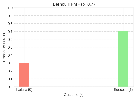

The Binomial Distribution: Bernoulli’s Ambitious Sibling

If Bernoulli is a single coin flip, Binomial is flipping that coin ‘n’ times and counting how many successes (e.g., heads) you got. Crucially, the trials must be independent, and the probability of success (p) must be the same for each trial.

Real-World Examples:

Number of students who pass an exam out of a class of 30, if each has a 70% chance of passing.
Number of heads in 10 coin flips.
Number of defective light bulbs in a batch of 50, if each has a 5% chance of being defective.

Python in Action:

n_trials = 10   # Number of coin flips
p_binom_success = 0.5 # Probability of heads for a fair coin
binom_dist = stats.binom(n_trials, p_binom_success)

# PMF for getting exactly 5 heads in 10 flips
prob_5_heads = binom_dist.pmf(5)
print(f"\nBinomial PMF (n={n_trials}, p={p_binom_success}):")
print(f"P(X=5 heads): {prob_5_heads:.3f}")

# Plotting the full PMF
k_values = np.arange(0, n_trials + 1)
probabilities_binom = [binom_dist.pmf(k) for k in k_values]

plt.figure(figsize=(8, 5))
plt.bar(k_values, probabilities_binom, color='skyblue', width=0.7)
plt.title(f'Binomial PMF (n={n_trials}, p={p_binom_success})')
plt.xlabel('Number of Successes (k)')
plt.ylabel('Probability P(X=k)')
plt.xticks(k_values)
plt.grid(True, axis='y', linestyle='--', alpha=0.7)
plt.show()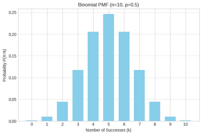

The Poisson Distribution: The “Event Counter” for Intervals

This distribution models the number of times an event occurs within a fixed interval of time or space, given that these events occur with a known constant mean rate and independently of the time since the last event. It’s the “how many?” distribution.

Real-World Examples:

Number of emails you receive per hour.
Number of customers arriving at a popular Chaat stall in Mysuru between 6 PM and 7 PM.
Number of typos on a page of a book.
Number of radioactive decays in a second.

Python in Action:

lambda_rate = 3  # Average number of emails per hour
poisson_dist = stats.poisson(lambda_rate)

# PMF for receiving exactly 2 emails in an hour
prob_2_emails = poisson_dist.pmf(2)
print(f"\nPoisson PMF (lambda={lambda_rate}):")
print(f"P(X=2 emails): {prob_2_emails:.3f}")

# Plotting the full PMF (up to a reasonable number)
k_values_poisson = np.arange(0, lambda_rate * 3 + 2) # Plot a bit beyond the mean
probabilities_poisson = [poisson_dist.pmf(k) for k in k_values_poisson]

plt.figure(figsize=(8, 5))
plt.bar(k_values_poisson, probabilities_poisson, color='lightcoral', width=0.7)
plt.title(f'Poisson PMF (lambda={lambda_rate})')
plt.xlabel('Number of Events (k)')
plt.ylabel('Probability P(X=k)')
plt.xticks(k_values_poisson)
plt.grid(True, axis='y', linestyle='--', alpha=0.7)
plt.show()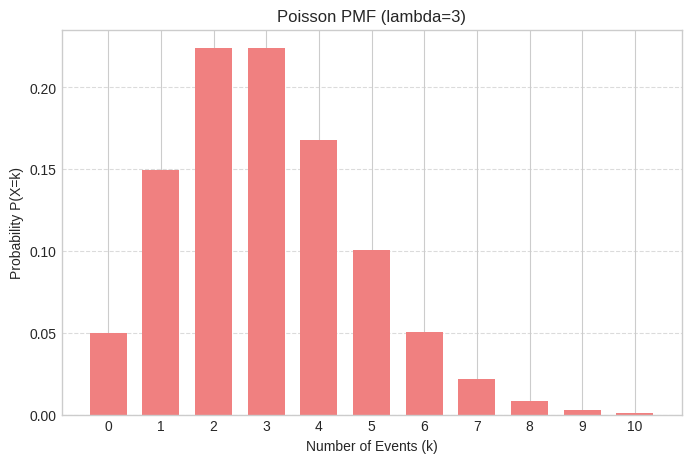

The Discrete Uniform Distribution: The Egalitarian

The Gist: The simplest of them all (conceptually, anyway). If you have ‘N’ possible outcomes, and each one is equally likely, you’ve got a discrete uniform distribution. Real-World Examples:

Rolling a fair six-sided die ($P(1)=P(2)=…=P(6)=\frac{1}{6}$).
Drawing a random card from a standard deck ($P(\text{any specific card})=\frac{1}{52}$).
Randomly picking an answer in a multiple-choice question you have absolutely no clue about (assuming 4 options, $P(\text{any option})=\frac{1}{4}$). This is generally not a recommended exam strategy, by the way. 🙃

Python in Action:

low = 1  # Lowest outcome of a die roll
high = 7 #randint is exclusive for the high parameter, so 7 means up to 6
uniform_dist = stats.randint(low, high)

# PMF for rolling any specific number (e.g., a 3)
prob_roll_3 = uniform_dist.pmf(3)
print(f"\nDiscrete Uniform PMF (for a fair die, outcomes 1-6):")
print(f"P(X=3): {prob_roll_3:.3f}") # Should be 1/6 = 0.167

# Plotting the PMF
outcomes_uniform = np.arange(low, high)
probabilities_uniform = [uniform_dist.pmf(k) for k in outcomes_uniform]

plt.figure(figsize=(8, 5))
plt.bar(outcomes_uniform, probabilities_uniform, color='mediumpurple', width=0.7)
plt.title(f'Discrete Uniform PMF (Fair Die)')
plt.xlabel('Outcome (k)')
plt.ylabel('Probability P(X=k)')
plt.xticks(outcomes_uniform)
plt.yticks(np.arange(0, 0.21, 0.05)) # Adjust y-ticks for clarity
plt.grid(True, axis='y', linestyle='--', alpha=0.7)
plt.show()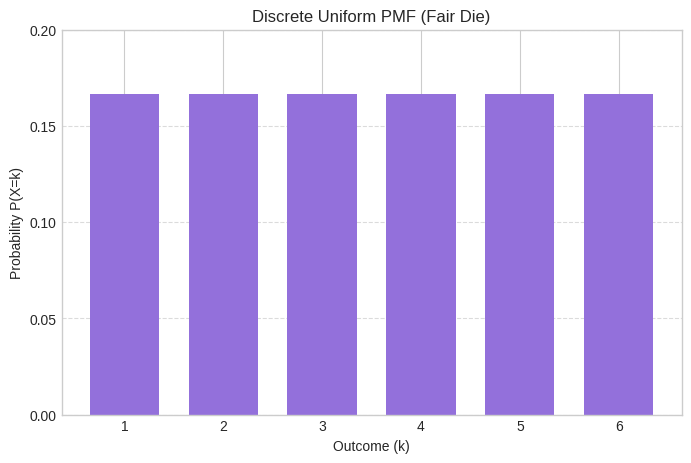

A Walking Tour of Popular Discrete Distributions

Below we introduce each distribution, spotlight a real scenario, and—because a little technical depth always comes handy—note its expectation $E[X]$ and variance $\text{Var}(X) $ . Code samples follow in the next section

Distribution	Use Case	PMF	$E[X]$	$\text{Var}(X) $	Wit‑Bit
Bernoulli(p)	Coin flip, binary classification	$p^x(1-p)^{1-x}$ $\text{for } k \in [1, 0]$	$p$	$p(1-p)$	The “yes/no” switch your recommender system toggles 1 B times a day.
Binomial(n,p)	Email batch success	$$ \binom{n}{x}p^x(1-p)^{n-x} $$	$np$	$np(1-p)$	Your inbox spam filter’s perspective on life: 0 = peace, $n$= apocalypse.
Geometric(p)	Number of tries until first bug‑free compile	$$(1-p)^{x-1}p $$	$$\frac{1}{p}$$	$$\frac{1-p}{p^2}$$	DevOps’ emotional roller coaster.
Negative Binomial(r,p)	Hits until r home runs	$$\tbinom{x-1}{r-1}(1-p)^{x-r}p^r $$	$$\frac{r}{p}$$	$$\frac{r(1-p)}{p^2}$$	Baseball fans call it “patience”; statisticians call it variance.
Poisson(λ)	Website hits per second	$$\frac{e^{-\lambda}\lambda^x}{x!}$$	$$\lambda$$	$$\lambda$$	The Internet at 2 a.m.: λ ≈ 0.1, unless you run a cat‑video site.
Discrete Uniform({1,…,k})	Random password digit	$$\frac{1}{k}$$	$$\frac{k+1}{2}$$	$$\frac{k^2 – 1}{12}$$	The fairest of them all; Snow White would approve.
Categorical(π₁…πₖ)	Next‑word in LLM	$$\pi_x$$	—	—	Every token armed with its own fanbase.
Multinomial(n,π)	Bag‑of‑words counts	$$\frac{n!}{\prod x_i!}\prod π_i^{x_i}$$	$$n\pi_x$$	$$n\pi_i(1-\pi_i)$$	Word‑count analytics, minus Shakespeare’s flair.
Zipf(s,N)	Word frequency rank	$$\frac{1/r^s}{H_{N,s}}$$	—	—	Proof the rich (words) get richer—“the” never sleeps.

(We skipped hypergeometric and friends for space—but feel free to invite them to your data party.)

PMFs Inside AI Models

Right, let’s connect this to the whirring brains of Artificial Intelligence. PMFs aren’t just for statistics class; they’re baked into the DNA of many AI algorithms.

Classification Task

Imagine an AI trying to classify an image: “Is this a picture of a cat, a dog, or a particularly fluffy idli?” For a given image, the AI needs to output its confidence for each class. The softmax function, often found at the tail end of neural network classifiers, takes the raw scores from the network and transforms them into a set of probabilities that sum to 1. What does that sound like? A PMF! Each class is a discrete outcome, and the AI assigns a probability to it.

$P(class=cat∣image)=0.7$
$P(class=dog∣image)=0.2$
$P(class=idli∣image)=0.1 $This PMF then guides the AI’s decision.

Reinforcement Learning (RL)

In RL, an agent often has a discrete action space – a specific set of actions it can take (e.g., “move left,” “move right,” “jump”). The agent’s “policy” can be a PMF that tells it the probability of choosing each action in a given state. “In this situation, there’s a 60% chance ‘move right’ is the best, 30% ‘jump’, and 10% ‘scream in binary’.”

Natural Language Processing (NLP)

When an AI is trying to understand or generate language, it’s dealing with discrete units – words (or tokens, sub-words). A basic language model trying to predict the next word in “The weather in Mysuru is ____” will essentially calculate a PMF over its entire vocabulary. “Sunny” might get a high probability, “cloudy” a decent one, and “banana” a very, very low one (unless it’s a very avant-garde weather report).

Attention Mechanisms (The “Focus” Enabler!)

And speaking of clever AI, let’s not forget Attention Mechanisms – the magic behind how models like Transformers decide what parts of that lengthy document or sentence are actually important! We’ve seen how softmax gives us a PMF for classification; attention mechanisms use a similar trick. They calculate relevance scores for different input words (tokens) and then normalize these scores (often using that same softmax function!) to create a set of attention weights. These weights, all positive and summing to 1, form a PMF across all the input tokens! This “attention PMF” tells the model where to “focus” its processing power, allowing it to grasp long-range dependencies and understand context much more effectively. It’s like giving the AI a smart, probabilistic highlighter pen.

Spotlight on Generative AI

This is where PMFs truly shine and why I wanted to give them a special shout-out in the context of Generative AI. Generative AI is all about creating new content – text, music, images, even code – that resembles the data it was trained on.

When Generative AI models are tasked with creating discrete sequences (like text, or symbolic music where notes are discrete units), PMFs are the engine driving the creative process, step-by-step:

The Autoregressive Idea: Many generative models for sequences work “autoregressively.” This fancy term just means they generate one element at a time, and each new element depends on the ones generated before it. Think of writing a story word by word. At each step, given the current context (e.g., “The cat sat on the…”), the Large Language Model (LLM) first computes raw scores called logits for every word in its vocabulary (which could be 50,000 words or more!). These logits aren’t probabilities yet. To turn them into a usable PMF, they’re fed through the softmax function, often with a twist called “temperature” (T): $$P(\text{next_token}_i | \text{context}) = \frac{e^{\text{logit}_i / T}}{\sum_j e^{\text{logit}_j / T}}$$ This resulting $$P(\text{next_token}_i | \text{context})$$ is our PMF for the next token! The temperature T is a crucial knob:
- High T (e.g., >1): Makes the PMF flatter, increasing randomness and “creativity.” The AI might pick less obvious words.
- Low T (e.g., <1, towards 0): Makes the PMF sharper, favoring high-probability words, leading to more focused, sometimes repetitive, output. T=1 is standard softmax.
Spinning the Roulette Wheel (Sampling): Once we have this PMF (let’s call it probs), the model doesn’t just pick the word with the absolute highest probability every time (that’s called greedy decoding, and it’s often boring). Instead, it samples from this PMF. It’s like spinning a roulette wheel where the size of each slot is proportional to the token’s probability. In PyTorch-like pseudocode, this might look like:

 logits = model(context) # Get raw scores from the LLM for all ~50k vocab words 
probs = torch.softmax(logits / T, dim=-1) # Convert to PMF with temperature 
next_token_id = torch.multinomial(probs, num_samples=1) # Spin the wheel!

This torch.multinomial function effectively performs that weighted random choice, giving us the ID of the next token.

Smarter Sampling: Top-k & Nucleus (Top-p) Tricks: Just sampling from the raw PMF can sometimes lead to… unexpected results. Imagine your AI is telling a knock-knock joke and suddenly veers off with “Platypus!” because “Platypus” had a tiny, non-zero probability in the PMF for that step. To prevent such delightful absurdities (or to encourage them, depending on your goal!), we use smarter sampling strategies that prune the PMF:
- Top-k Sampling: Only consider the k tokens with the highest probabilities. Create a new PMF by renormalizing these k probabilities, then sample from this smaller set. If k=50, you’re only choosing from the 50 most likely next words.
- Nucleus (Top-p) Sampling: Instead of a fixed k, choose the smallest set of tokens whose cumulative probability mass is greater than or equal to some value p (e.g., p=0.9). Then, renormalize their probabilities and sample from this “nucleus” of high-probability tokens. This is adaptive – if the model is very certain about the next few words, the nucleus will be small; if it’s uncertain, the nucleus can be larger.
- Both these methods help to avoid the “long tail” of low-probability tokens sabotaging coherence, giving us more control over the generation process.
Repeat! The chosen word is added to the sequence, becomes part of the new context, and the model goes back to step 2 to predict a PMF for the next word. This continues until a desired length is reached or an “end-of-sequence” token is generated.

This isn’t just for text!

Symbolic Music Generation: Generating a melody note by note. The model predicts a PMF over all possible next notes (C, D, E#, rest, etc.) given the previous notes, and then samples.
Generating Code: Similar idea, predicting the next token or character in a programming language.
Discrete Latent Variables: Even in some image generation models, if they use a discrete latent space (a kind of compressed representation that is categorical), PMFs will be involved in choosing which category to represent.
PMFs in Image Models? You might think images are purely continuous (pixel values). While largely true, PMFs can sneak in even there! In some diffusion models or systems using classifier-free guidance, decisions about discrete noise levels to apply or discrete choices in guidance steps can be governed by learned or implicit PMFs. So, even in visually continuous generation, underlying discrete probabilistic choices, modeled by PMFs, can play a role.

Without PMFs to guide the selection of each discrete element, generative AI for sequences would be like trying to write a novel by randomly picking words from a dictionary – pure chaos. The PMF provides the probabilistic intelligence to make coherent, creative, and contextually relevant discrete choices.

Common Pitfalls & Misconceptions

Navigating the world of PMFs in AI isn’t always a walk in the park. Here are a few banana peels to watch out for:

Probabilities smaller than 1e-5 are safe to ignore.
- Nope! While individually tiny, the cumulative effect of many rare events can be massive. Ask any risk manager or someone whose LLM just generated something wildly inappropriate because a “rare” token sequence got sampled. In large vocabularies, the tail of the PMF matters.
PMF and PDF are basically interchangeable.
- Only if you think a refreshing glass of tender coconut water and a shot of espresso are the same beverage! They both quench a thirst, but they’re fundamentally different.
  - PMF → Discrete Random Variables (countable, separate outcomes like dice rolls, word choices). Gives actual probability at each point.
  - PDF → Continuous Random Variables (measurable outcomes like height, temperature). Gives probability density; you integrate over a range to get probability.
Softmax always makes probabilities sum to 1, so if my model uses softmax, the probabilities are ‘correct’ and training will fix everything.

The Grand Finale: PMFs – Small Math, Mighty Impact!

So, there you have it! The Probability Mass Function, from its humble beginnings with dice rolls to powering the sophisticated “next-token roulette” in giant language models. It’s a cornerstone concept that gives us a clear, actionable way to understand and work with discrete uncertainties.

In the world of AI, especially the exciting frontier of Generative AI, PMFs are the quiet enablers of creativity and control. They provide the structured randomness, the intelligent choice mechanism, that allows machines to compose, write, and generate sequences that can inform, entertain, and sometimes, make us laugh (or scratch our heads at a platypus in a knock-knock joke).

The next time you interact with a chatbot, see AI-generated art, or marvel at machine-composed music with discrete notes, remember the PMF. It’s diligently working behind the scenes, shaping possibilities, assigning probabilities, and making those tiny, crucial discrete choices that add up to something remarkable.

Has this deeper dive into PMFs and their role in things like temperature scaling, top-k/top-p sampling, and even image models sparked new ideas? What are some common pitfalls you’ve encountered with probabilities in AI?

Drop your thoughts in the comments below – let’s get the conversation rolling!

Please follow and like us: