Is Your Model's Accuracy Genuine? A Test to Be Sure

The Feynman Test for Not Fooling Yourself About Test-Set Accuracy

“The first principle is that you must not fool yourself — and you are the easiest person to fool.” — Richard Feynman

I keep Feynman’s line taped, metaphorically, to the inside of every model I train. Because here is the uncomfortable truth about that beautiful 94% you just saw print out on your test set: a number, on its own, tells you almost nothing. A stopped clock is right twice a day. A coin that always shouts “heads” is correct half the time. And a model that has quietly memorised a spurious shortcut can look like a genius right up until it meets the real world and falls flat on its face.

So let me walk you through how I actually interrogate a high accuracy score — the way a slightly paranoid scientist should. We will build the idea from the ground up: what “due to chance” even means, how much data changes the answer, and why balanced and imbalanced datasets demand completely different verdicts on the same number.

First, what do we mean by “due to chance”?

There are really two very different worries hiding inside this question, and untangling them is half the battle.

Worry 1 — Sampling luck. Your test set is a finite sample drawn from some larger population. Even a mediocre model can score well on a particular sample simply because that sample happened to contain easy examples. If you had drawn a different test set, the score might have been worse. This is the statistician’s “chance”: the variability that comes from measuring on a limited number of points.

Worry 2 — A model that is no better than guessing. Here the concern is that the model has learned nothing useful, and its accuracy is merely what any trivial strategy — always predict the majority class, or flip a weighted coin — would achieve. The score is “real” in the sense that it is reproducible, but it is meaningless because a brainless baseline matches it.

Genuine accuracy has to survive both interrogations. It must be high enough that sampling luck alone is an implausible explanation, and high enough to clear the bar set by a trivial baseline. Let us take them one at a time.

The mental model: accuracy is a coin-flip experiment

Think of evaluating on a test set of n examples as flipping n coins. Each prediction is either right (heads) or wrong (tails). If the model’s true accuracy — its accuracy over the whole population — is p, then the number of correct answers follows a binomial distribution. This single idea unlocks almost everything else.

The standard deviation of the observed accuracy is

$$\sigma = \sqrt{\frac{p(1-p)}{n}}$$

Stare at that denominator. The uncertainty shrinks as $\sqrt{n}$. Quadruple your test set and you halve your error bars. This is why how much data you have is not a footnote — it is the whole story of how much you should trust the number.

Condition 1: You have very little test data

Suppose your test set has only 50 examples and you score 90%. Feels great. But let’s put honest error bars on it. With $p \approx 0.9$ and $n = 50$:

$$\sigma = \sqrt{\frac{0.9 \times 0.1}{50}} \approx 0.042$$

A rough 95% interval is $0.9 \pm 1.96\sigma \approx 0.9 \pm 0.083$ — roughly 82% to 98%. For such small samples I prefer the Wilson score interval, which behaves far better near the extremes than the naive formula above:

from statsmodels.stats.proportion import proportion_confint

# 45 correct out of 50
low, high = proportion_confint(count=45, nobs=50, alpha=0.05, method="wilson")
print(f"95% CI: [{low:.3f}, {high:.3f}]")   # ~[0.786, 0.957]

The lesson: on tiny test sets, a stunning accuracy is compatible with a fairly ordinary true accuracy. The number is not lying, but it is whispering when you wanted it to shout. My rules of thumb when data is scarce:

Report the confidence interval, never the point estimate alone. A single number without error bars is a rumour, not a result.
Use k-fold cross-validation (or repeated k-fold) so that every example takes a turn as test data. This makes maximal use of scarce data and gives you a spread of scores whose variance you can inspect. Beware, though: CV fold scores are not independent (training sets overlap heavily), so the naive standard error across folds is optimistic. The Nadeau–Bengio corrected variance is the honest fix for repeated CV.
Consider the humble binomial test (below) to ask directly: could a coin have done this?

Condition 2: Balanced data — the friendly case

When your classes are roughly equal in size, accuracy is a reasonably honest summary, and the key question becomes: is my model beating chance?

Here the chance baseline is clean. For two balanced classes, random guessing scores 50%. So we ask: given my n test points, how surprised should I be to see this many correct if the model were truly no better than a coin? That is a one-sided binomial test.

from scipy.stats import binomtest

# 88 correct out of 100, null hypothesis = 50% (chance for balanced 2-class)
res = binomtest(k=88, n=100, p=0.5, alternative="greater")
print(f"p-value: {res.pvalue:.2e}")   # astronomically small -> not chance

If that p-value is tiny, sampling luck against a coin is a wildly implausible explanation, and you can say the model is genuinely better than chance. But — and this matters — “better than a coin” is a low bar. Clearing it is necessary, not sufficient, for a good model.

The most robust and assumption-free tool I reach for on balanced data is the permutation test. The logic is delicious in its honesty: if your labels carry no information the model can exploit, then shuffling the labels and retraining should give you roughly the same accuracy. So we build the null distribution empirically by destroying the label–feature relationship many times over.

from sklearn.model_selection import permutation_test_score, StratifiedKFold

score, perm_scores, pvalue = permutation_test_score(
    estimator, X, y,
    scoring="accuracy",
    cv=StratifiedKFold(5, shuffle=True, random_state=0),
    n_permutations=1000, random_state=0,
)
print(f"True score: {score:.3f}")
print(f"Chance level (mean of permutations): {perm_scores.mean():.3f}")
print(f"p-value: {pvalue:.4f}")

The p-value is simply the fraction of shuffled runs that matched or beat your real score (with a +1 correction in numerator and denominator). If out of 1000 shuffles almost none reach your accuracy, your model has found real structure. If half of them do, your “94%” is exactly what a label-blind process produces — a sobering thing to discover, but far better to discover it now than in production.

Condition 3: Imbalanced data — where accuracy lies to your face

This is where most people fool themselves, so I will be blunt. On imbalanced data, accuracy is close to useless as a standalone metric.

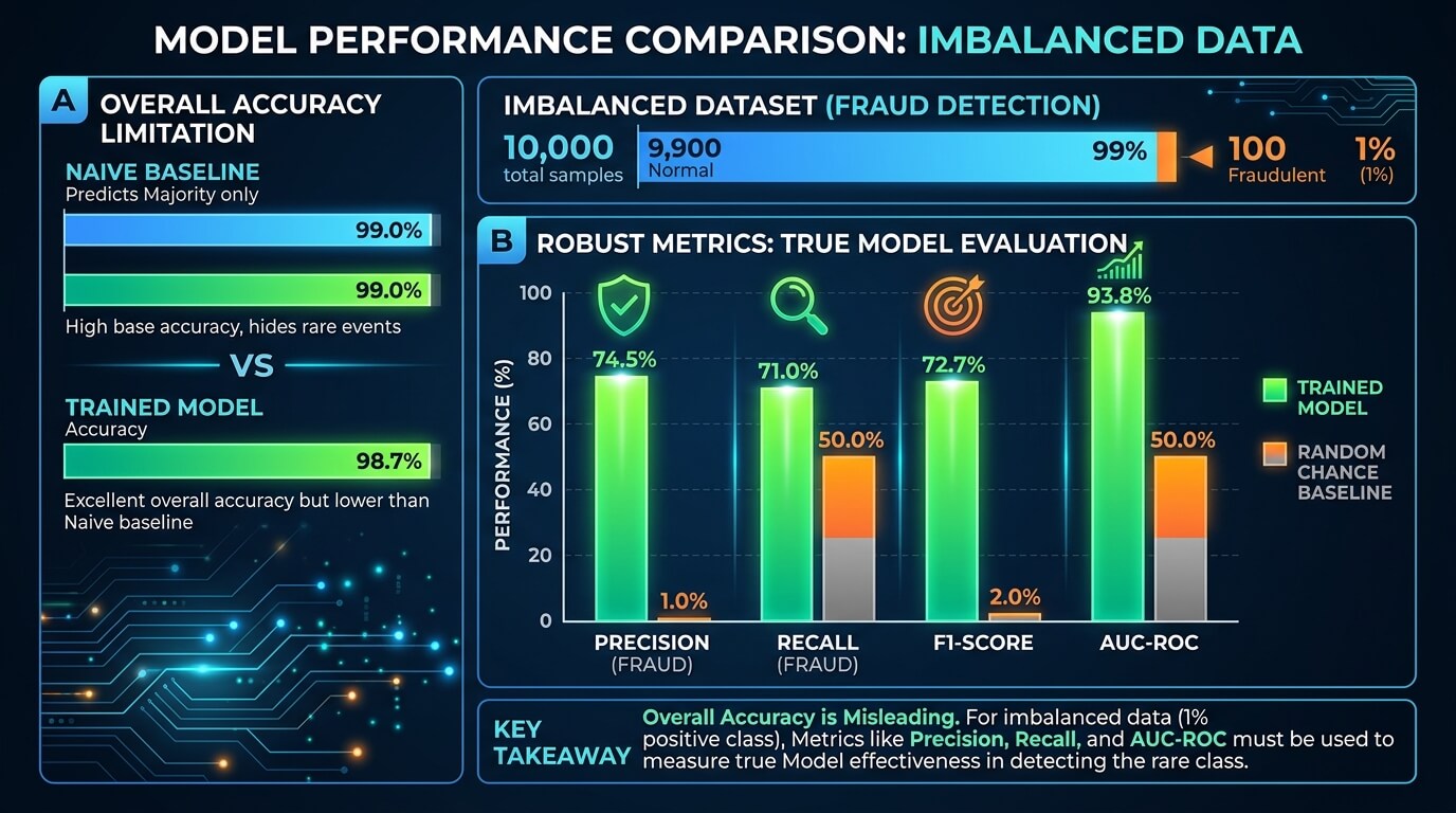
Picture fraud detection where 99% of transactions are legitimate. A model that predicts “legitimate” for everything scores 99% accuracy and catches exactly zero frauds. It is worthless, yet the accuracy number is dazzling. The chance baseline is no longer 50% — it is the No-Information Rate (NIR), the proportion of the majority class. Your 99% must be compared against that 99%, not against 50%, and suddenly it is unimpressive.

The binomial test adapts naturally: test against $p = \text{NIR}$, not $p = 0.5$.

from scipy.stats import binomtest
# 950 correct of 1000, but majority class is 95% of the data
res = binomtest(k=950, n=1000, p=0.95, alternative="greater")
print(f"p-value vs no-information rate: {res.pvalue:.3f}")  # ~0.5 -> no better than guessing majority

But the deeper fix is to stop looking at accuracy at all and use metrics that cannot be gamed by ignoring the minority class:

Precision, recall, and F1 — computed per class, and especially for the minority class you actually care about. Recall answers “of the real frauds, how many did I catch?”; precision answers “of my fraud alarms, how many were real?”
Balanced accuracy — the average of recall across classes, which collapses to chance (50% for two classes) for the majority-guessing model, stripping away the illusion.
Matthews Correlation Coefficient (MCC) — my personal favourite single number for imbalanced problems. It uses all four cells of the confusion matrix and only scores high when the model does well on both classes:

$$\text{MCC} = \frac{TP \cdot TN – FP \cdot FN}{\sqrt{(TP+FP)(TP+FN)(TN+FP)(TN+FN)}}$$

It ranges from −1 (perfectly wrong) through 0 (random) to +1 (perfect). The majority-guessing fraud model scores MCC = 0, which is exactly the honesty we want.

Cohen’s kappa — measures agreement beyond chance, $\kappa = (p_o – p_e)/(1 – p_e)$, where $p_o$ is observed accuracy and $p_e$ is the accuracy expected by chance given the class frequencies. Kappa near 0 means “no better than chance” even if raw accuracy looks high.
ROC-AUC and, better still for heavy imbalance, PR-AUC (area under the precision–recall curve), which focuses squarely on the rare positive class.

from sklearn.metrics import (balanced_accuracy_score, f1_score,
                             matthews_corrcoef, cohen_kappa_score,
                             classification_report)

print(classification_report(y_test, y_pred))          # per-class precision/recall/F1
print("Balanced acc:", balanced_accuracy_score(y_test, y_pred))
print("MCC:", matthews_corrcoef(y_test, y_pred))
print("Kappa:", cohen_kappa_score(y_test, y_pred))

If you take one thing from this section: always compute a DummyClassifier baseline. It costs three lines and it is the single most effective antidote to self-deception on imbalanced data.

from sklearn.dummy import DummyClassifier
dummy = DummyClassifier(strategy="most_frequent").fit(X_train, y_train)
print("Baseline accuracy:", dummy.score(X_test, y_test))

If your fancy model barely edges out most_frequent, you do not have a model — you have a class-frequency counter wearing a lab coat.

Comparing two models: is B really better than A?

Often the real question is not “is it better than chance” but “is my new model genuinely better than the old one, or did it win by a coin-flip’s margin?” For two classifiers evaluated on the same test set, the correct tool is McNemar’s test, which looks only at the examples where the two models disagree.

from statsmodels.stats.contingency_tables import mcnemar
import numpy as np

# n01 = A wrong & B right ; n10 = A right & B wrong
correct_A = (pred_A == y_test)
correct_B = (pred_B == y_test)
n01 = np.sum(~correct_A & correct_B)
n10 = np.sum(correct_A & ~correct_B)
table = [[0, n01], [n10, 0]]
print(mcnemar(table, exact=False, correction=True))

If model B’s wins over A are not statistically distinguishable from A’s wins over B, then B’s higher headline accuracy is likely noise. For comparing across cross-validation folds, use a paired test but apply the Nadeau–Bengio correction to the variance, because the folds share training data and the naive paired t-test will declare victories that aren’t there.

The silent killers: leakage and test-set reuse

Even a statistically significant, baseline-beating score can be a mirage if the experimental setup is broken. Two mistakes I hunt for relentlessly:

Data leakage. If information from the test set sneaks into training — because you scaled or imputed using statistics computed over the whole dataset, or because near-duplicate rows straddle the split, or because a feature secretly encodes the target — then your test set is no longer a fair exam. Fit every preprocessing step inside a pipeline on the training fold only:

from sklearn.pipeline import make_pipeline
from sklearn.preprocessing import StandardScaler
pipe = make_pipeline(StandardScaler(), estimator)   # scaler fit only on train folds

Test-set reuse (the multiple-comparisons trap). If you tune hyperparameters against the test set, or peek at it fifty times, you are slowly overfitting to the test set itself. Eventually one configuration looks brilliant purely by chance — the statistical version of torturing the data until it confesses. Keep a truly held-out set that you touch once, and do all tuning on a separate validation split or via nested cross-validation. The most convincing evidence of genuine performance is strong results on data collected at a different time or place — a temporal or out-of-distribution test.

Putting it together: my checklist

When someone shows me a high accuracy and asks “is it real?”, I run down this list, in order:

How big is the test set? Attach a Wilson confidence interval. Small n → wide interval → be humble.
What is the class balance? If imbalanced, mentally delete the accuracy number and look at balanced accuracy, per-class recall, F1, MCC, and PR-AUC instead.
What does a DummyClassifier score? Establish the no-information rate before celebrating anything.
Does it beat chance statistically? Binomial test against the right baseline (0.5 or the NIR), or better, a permutation test for an assumption-free null.
Is a rival model actually beaten? McNemar’s test on the same test set; Nadeau–Bengio-corrected paired test across CV folds.
Is the pipeline clean? No leakage, no test-set reuse, preprocessing fit only on training data.
Does it hold up out-of-distribution? The ultimate proof is generalisation to genuinely new data.

Pass all seven and I will believe your accuracy is real. Skip any of them and you may simply be, as Feynman warned, the easiest person to fool.

A few resources I recommend

If you want to go deeper, the two books I hand to my students most often are An Introduction to Statistical Learning by James, Witten, Hastie and Tibshirani — the single best on-ramp to the bias, variance, and resampling ideas underlying everything above — and Aurélien Géron’s Hands-On Machine Learning with Scikit-Learn, Keras and TensorFlow for the practical, code-first treatment of evaluation and pipelines. Both are widely available (including on Amazon), and both earned their place on my shelf long before I ever recommended them here.

Disclosure: some of the book links above are Amazon affiliate references, which means I may earn a small commission if you purchase through them — at no extra cost to you. I only ever recommend books I genuinely use and trust.

Reflection questions — test your own understanding

Your model scores 97% on a 30-sample test set. Before you celebrate, what is the approximate 95% confidence interval, and what does its width tell you?
A colleague reports 91% accuracy on a dataset that is 90% one class. What single baseline would instantly reframe that result, and what metrics would you ask to see instead?
Why does a permutation test give a more trustworthy “chance level” than simply assuming 50%? When would the two disagree?
You improve accuracy from 88.0% to 88.6% by switching models. Which test tells you whether that gain is real, and what feature of the data does it exploit?
Explain in one sentence, to a bright 12-year-old, why measuring on more test examples makes you more confident — using the coin-flip picture.

Work through those and you will have internalised the difference between a number that looks good and a result you can stand behind.

About the author

I’m Dr Amita Kapoor — an AI researcher, educator, and author who has spent two decades teaching machines to learn and humans to understand the machines. I’ve written several books on deep learning and reinforcement learning, and I care deeply about explanations that are simple without being wrong.

I’m the founder of NePeur (nepeur.com), where I build and consult on practical, trustworthy AI systems, and a co-founder of Retured, where we work at the intersection of technology and sustainability — using AI to help the planet, not just the leaderboard. If this way of thinking about rigour resonates with you, come find me there.

Please follow and like us: