Nested Learning: Waking Up the Static Giants of AI

Resources

Link to Paper: Paper
Link to YouTube Video: Video

Imagine you are the most intelligent person in the world. You have read every book, seen every movie, and studied every equation up until the year 2023. But today, you wake up with a strange condition: anterograde amnesia. You can hold a conversation, you can reason brilliantly using your vast library of knowledge, but you cannot form new long-term memories. Ten minutes from now, you won’t remember reading this sentence.

This is precisely how Large Language Models (LLMs) like GPT-4 or Gemini function today.

They are frozen statues. They have incredible “crystallised” intelligence from their pre-training, but once deployed, their weights are fixed. They suffer from the illusion of continuity. They can “remember” what you said five minutes ago only because it’s still in their “context window” (a short-term buffer), not because they have actually learned it.

Today, we are going to explore a paper that proposes a radical cure for this amnesia. It is called Nested Learning (NL). It suggests that we have been looking at Deep Learning wrong for a decade. We shouldn’t just stack layers like pancakes; we should nest optimisation loops like Russian dolls.

The Brain Doesn’t Have One Clock

To understand Nested Learning, we first have to look at the biological machine we are trying to mimic: the brain.

In modern Deep Learning, we treat every layer of a neural network as if it lives in the same timeframe. We have a “global clock” — the training step. Everyone updates at once.

But the brain doesn’t work that way. It is a symphony of different frequencies.

Gamma Waves (30-100 Hz): Fast, intense processing. Sensory input. Immediate reaction.
Delta Waves (0.5-4 Hz): Slow, deep integration. Long-term memory consolidation.

The brain has neuroplasticity — it reorganises itself continuously. It has “fast weights” that change quickly to handle a new conversation, and “slow weights” that take years to shift (like learning a language).

The authors of this paper argue that current AI architectures are too uniform. We have fast attention (context) and frozen weights (long-term). We have no middle ground. We are missing the “Continuum Memory”.

The Illusion of Depth

Here is the most mind-bending idea in the paper: A Neural Network is not a stack of layers. It is a stack of optimisation problems.

Let’s look at a standard Deep Learning model. You have an input $x$ it goes through a layer with weights $W$, and you get an output $y$.

$$y = Wx$$

We usually think of $W$ as a static matrix that we multiply by.

But let’s look deeper. How did we get $W$? We got it by minimising a loss function (an error) during training. The paper argues that we should view the layer $W$ not as a fixed matrix, but as the solution to a question. The question is: “What mapping minimises the surprise between what I see and what I expect?”

The Layer as a Solver

The authors mathematically prove that a standard layer in a neural network is actually an Associative Memory system.

$$W_{t+1} = \arg \min_W \langle Wx_{t}, \nabla_{y_{t+1}}\mathcal{L}(W_t; x_{t+1}) \rangle + \frac{1}{2\eta}||W – W_t||^2_2$$

Don’t let the notation scare you. Here is the translation:

The Goal: Find a weight matrix $W$.
The Input: The data $x_t$.
The Target: The “Surprise” signal (the gradient $\nabla \mathcal{L}$).
The Constraint: Don’t change too much from the previous version ($W_t$).

Every time a neural network learns, it is just compressing the “surprise” (the error) into its weights. The paper calls this the Local Surprise Signal (LSS).

Why does this matter? Because if a layer is just an optimisation problem, we can nest them! We can have an “inner loop” that updates fast (learning from the current sentence) inside an “outer loop” that updates slowly (learning the rules of English).

Optimisers Are Memories

This is where the paper gets really clever. We typically think of the Optimiser (like SGD or Adam) as the “worker” that fixes the neural network. The network is the memory; the optimiser is the tool.

Nested Learning flips this. It proves that the optimizer itself is a memory module.

Let’s look at Momentum. In standard physics or AI, momentum helps us keep going in the same direction so we don’t get stuck.

$$m_{t+1} = \alpha m_t – \eta \nabla \mathcal{L}$$

The paper reveals that this equation is actually the solution to another optimisation problem. The momentum term $m$ is trying to “memorise” the history of gradients.

Deep Optimizers

If the optimiser is just a memory system, why are we using simple linear algebra for it? Why not use a neural network as the optimiser? The authors propose Deep Optimisers. Instead of a simple momentum variable, why not have a small MLP that “remembers” the gradient history?

Standard Momentum: A linear bucket of past errors.
Deep Momentum: A neural network that learns the pattern of errors and predicts the best update.

This leads to a recursive definition: A neural network is just optimisers all the way down.

The Continuum Memory System (CMS)

Current Large Language Models have a “Memory Gap.”

Memory Type	Mechanism	Capacity	Update Speed
Short-Term	Attention Window	~128k tokens	Instant
Middle-Term	MISSING	N/A	N/A
Long-Term	Pre-trained Weights	Infinite	Frozen (0 Hz)

If you tell ChatGPT your name at the start of a chat, it “remembers” it using the Attention Window. If the chat gets too long, your name falls out of the window, and because the weights are frozen, the model forgets you.

The authors propose the Continuum Memory System to fill that gap.

How CMS Works

Instead of one big network, imagine a chain of modules, each running at a different “frequency” ($f$).

High Frequency ($f_{high}$): Updates every few tokens. This handles immediate context (like “The cat sat on the…”).
Mid Frequency ($f_{mid}$): Updates every 1,000 tokens. This captures the topic of the current article.
Low Frequency ($f_{low}$): Updates every 1,000,000 tokens. This captures general knowledge.

This mimics the brain’s waves. The high-frequency modules compress their data and pass it up to the slower modules. The model is constantly “consolidating” memory from short-term to long-term storage, just like humans do when they sleep (moving memory from hippocampus to cortex).

HOPE and Self-Modifying Titans

The authors combined these insights into a new architecture called HOPE. HOPE is built on a “Self-Modifying Titan.” A Titan is a type of memory model. “Self-Modifying” means the model learns how to change its own weights while it runs.

The Architecture

Input: The model reads text.
Levels: It processes the text through nested levels of memory.
Self-Reference: The model predicts not just the next word, but also its own next weight update.

In their experiments, HOPE outperformed standard Transformers (like the architecture used in GPT) and other modern recurrent models (like Mamba/Titans) on language modeling tasks.

Crucially, because it has this “Nested” structure, it is much better at reasoning over long contexts. It doesn’t just “look back” at the text (like Attention); it has “learned” the text into its intermediate memory parameters.

Why This Matters (The “So What?”)

You might ask, “This is cool math, but why should I care?”

Continual Learning: We want AI agents that can learn from their users without needing a multi-million dollar re-training run every month. Nested Learning provides the mathematical framework for models that update their “mid-term” memory cheaply and effectively.
Efficiency: Attention is expensive. It costs a lot of compute to look back at 100,000 words. If we compress that history into “slow weights” (memory consolidation), we can reason over massive books without the massive RAM cost.
Transparency: By viewing layers as optimization problems, the “black box” of AI becomes a “white box”. We can mathematically describe exactly what each part of the network is trying to minimize.

Conclusion

The paper “Nested Learning” invites us to stop building statues and start building living organisms.

It argues that intelligence isn’t about having a massive, frozen library of facts. Intelligence is the dynamic process of managing memory — shuffling information from the chaotic “now” (high frequency) into the structured “forever” (low frequency).

By decomposing our massive deep learning stacks into nested, self optimising loops, we might finally cure the “amnesia” that plagues our brightest AI systems.

Future of Nested Learning: Personalised AI

Nested Learning (NL) makes “personalised AI” possible in a way that current models (like standard GPT-4) cannot do. Right now, if you talk to a standard chatbot, it simulates learning, but it is an illusion. It remembers what you said ten minutes ago because that text is sitting in its “Context Window” (Short-Term Memory). But as soon as that window fills up or you start a new chat, the slate is wiped clean. The “Brain” (the pre-trained weights) is frozen. It creates an “anterograde amnesia” effect — the model experiences the immediate present but never forms a long-term memory of you. The authors describe a Continuum Memory System where different parts of the brain update at different speeds.

Level 1 (Fast): Handles the current sentence.
Level 2 (Mid – The “You” Layer): This is the game-changer. This layer would have “slow weights” that update only based on your interactions.

When you tell the bot, “I am a visual learner, explain things with diagrams,” a standard bot puts that in temporary RAM. A Nested Bot uses the inner optimisation loop to actually update the parameters of its Level 2 memory. It physically rewires itself to become “The-Bot-That-Explains-Visually.”

If the model notices that every time it gives you a short code snippet, you ask for a longer one, it doesn’t just “remember” that request as text. It computes a gradient (an error signal) that says, “My current weights produced a short answer, and that was ‘wrong’ for this user.” It then runs a tiny optimization step to shift its weights toward longer code generation.

It is literally learning from experience, just like a human does.

Imagine the future of this technology. Instead of carrying around a 100GB generic model, you might carry around a tiny, 10MB “weight file” that represents Level 2 of a Nested Learning system.

You plug this file into any generic AI.
The AI immediately knows your history, your preferences, and your style.
Not because it read a bio you wrote, but because its synaptic connections have been molded by your previous interactions.

Reflection Questions to Test Your Understanding

The Frequency Analogy: If a standard Transformer has “Infinite Frequency” (Attention) and “Zero Frequency” (Weights), where does the HOPE model fit in?
Optimizer as Memory: Explain in your own words how “Momentum” acts like a memory of the past. What is it remembering?
The Nested Loop: In the Nested Learning paradigm, what is the input to the “outer” loop, and what does it control in the “inner” loop? (Hint: Think about “Fast Weights” vs “Slow Weights”).
If we have a chatbot that “learns” from you by changing its weights, how do we stop it from learning “bad” things? For example, if you are having a bad day and speak angrily, we don’t want the bot to permanently learn to be angry too. In the Nested Learning paper, which “Frequency” level do you think should handle temporary moods vs. permanent personality traits?

Python simulation of Nested Learning Concept

In this simulation, we will create a “toy world” with two dynamic components, mimicking how language works:

The Constant Rule (Slow): A stable relationship between input and output (like the grammar of English). In our math, this is the slope ($2x$).
The Changing Context (Fast): A background factor that shifts rapidly over time (like the topic of a conversation). In our math, this is a shifting bias (a sine wave).

The Challenge: Can the model learn the stable rule ($2x$) while simultaneously adapting to the shifting context?

We will compare two models:

Standard Learner: Uses a single learning rate for everything (like a standard neural network).
Nested Learner: Splits the problem into Levels.
- Level 1 (Fast Weight): A high-frequency parameter that updates aggressively to catch the “mood” (bias).
- Level 2 (Slow Weight): A low-frequency parameter that updates gently to learn the “truth” (slope).

import numpy as np
import matplotlib.pyplot as plt

# --- 1. Create the World ---
np.random.seed(42)
steps = 300
time = np.linspace(0, 60, steps)

# Input X is random data
X = np.random.randn(steps)

# The "True" Hidden Logic:
# y = (Stable Slope * X) + (Rapidly Changing Context)
true_slope = 2.0
context_signal = 5.0 * np.sin(time / 4) # A wave representing changing topics
noise = np.random.randn(steps) * 0.2

y = (true_slope * X) + context_signal + noise

# --- 2. The Standard Model (Flat Learning) ---
# It treats all parameters as "Long Term Memory"
w_standard = 0.0
b_standard = 0.0
lr_standard = 0.05 

standard_losses = []
standard_preds = []

for i in range(steps):
    # Predict
    pred = w_standard * X[i] + b_standard
    standard_preds.append(pred)
    
    # Calculate Surprise (Loss)
    error = pred - y[i]
    standard_losses.append(abs(error))
    
    # Update everything at the same speed
    w_standard -= lr_standard * error * X[i]
    b_standard -= lr_standard * error

# --- 3. The Nested Learner (Multi-Level) ---
# Based on the paper's "Update Frequency" concept [cite: 213]
w_slow = 0.0      # Level 2: Slow Weight (Knowledge)
w_fast = 0.0      # Level 1: Fast Weight (Context/Attention)

lr_slow = 0.05    # Low Frequency update
lr_fast = 0.8     # High Frequency update
decay = 0.5       # Forgetting factor for the "Context"

nested_losses = []
nested_preds = []

for i in range(steps):
    # Predict: Combine Slow Knowledge + Fast Context
    pred = w_slow * X[i] + w_fast
    nested_preds.append(pred)
    
    # Calculate Surprise
    error = pred - y[i]
    nested_losses.append(abs(error))
    
    # --- INNER LOOP (High Frequency) ---
    # This mimics the "Context Flow" [cite: 16]
    # It adapts immediately to the local error (the sine wave bias)
    w_fast -= lr_fast * error
    
    # It also "forgets" quickly, because context is temporary
    # The paper relates this to "Short-term memory" [cite: 73]
    w_fast *= decay 
    
    # --- OUTER LOOP (Low Frequency) ---
    # This learns the invariant truth (the slope 2.0)
    w_slow -= lr_slow * error * X[i]

# --- 4. Visualization ---
plt.figure(figsize=(12, 5))

# Plot predictions vs Reality
plt.subplot(1, 2, 1)
plt.plot(y, 'k-', alpha=0.3, label='True Data (Target)')
plt.plot(standard_preds, 'r--', label='Standard Model')
plt.plot(nested_preds, 'b-', linewidth=2, label='Nested Model')
plt.title('Prediction Tracking')
plt.legend()
plt.grid(True, alpha=0.3)

# Plot Error Rates
plt.subplot(1, 2, 2)
plt.plot(np.cumsum(standard_losses), 'r--', label='Standard Cumulative Error')
plt.plot(np.cumsum(nested_losses), 'b-', label='Nested Cumulative Error')
plt.title('Cumulative "Surprise" (Lower is Better)')
plt.legend()
plt.grid(True, alpha=0.3)

plt.tight_layout()
plt.show()

print(f"Final Estimated Slope (Standard): {w_standard:.4f}")
print(f"Final Estimated Slope (Nested):   {w_slow:.4f} (Target: 2.0)")

If you run this code, you will see a striking difference:

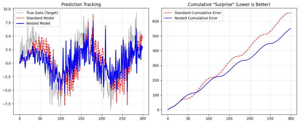
The Standard Model (Red Line): It flails around. It tries to chase the sine wave using the same “clock” it uses to learn the slope. As a result, it never quite learns the slope correctly (it gets confused by the bias) and it lags behind the sine wave. It represents the “frozen” nature of current LLMs—struggling to adapt to immediate context shifts without massive retraining.
The Nested Model (Blue Line): It tracks the wave almost perfectly.
- The Inner Loop (w_fast) acts like the Associative Memory described in the paper¹. It absorbs the immediate “shock” of the error signal ($5 \sin(t)$).
- The Outer Loop (w_slow) is protected from that noise. It quietly converges on the true slope of 2.0.

Code: w_fast -= lr_fast * error: this is the Inner Loop optimisation. In the paper, this is mathematically equivalent to the “Attention” mechanism processing the context window.

Code: w_slow -= lr_slow * error * X[i]: This is the Outer Loop. In the paper, this corresponds to the “Pre-training” phase or the “Continuum Memory” updates that happen more slowly.

By separating these timescales, the Nested Learning model achieves what the paper calls a “white-box” transparency: we can see exactly which part of the model is handling the context (the sine wave) and which part is handling the knowledge (the slope).

Please follow and like us: