
Imagine you’re trying to teach a machine the difference between a cat and a dog. You show it a picture of a cat, and it says, with 90% confidence, “That’s a cat.” Great! Now you show it a dog, and it says, with 60% confidence, “That’s a cat.” Not so great. The second guess is not just wrong; it’s also brimming with misplaced confidence. How do we teach the machine to be not only correct but also appropriately confident? How do we quantify the penalty for being both wrong and certain about it?
This is the central question answered by a cornerstone of modern machine learning: Binary Cross-Entropy (BCE), also called Log Loss. It’s a loss function, a mathematical tool for measuring the “cost” of a wrong prediction – that is exquisitely suited for any task that involves a simple binary choice: yes/no, 0/1, cat/dog, real/fake. Understanding BCE is fundamental to grasping how AI systems, from simple classifiers to the powerful engines of generative AI, learn to navigate a world of probabilities.
Let’s break down this elegant concept from its very foundations, see how it powers AI, and explore its specific, crucial roles in the sophisticated worlds of Generative AI and Large Language Models (LLMs).
What’s in a Guess? From Probabilities to Penalties
Let’s start with a simple task. We have an AI model that looks at emails and must decide if an email is spam (1) or not spam (0). A well-designed model won’t just output a rigid “spam” or “not spam.” Instead, it will output a probability—a number between 0 and 1 representing its confidence. For instance, it might say there’s a 0.95 probability that an email is spam.
Now, let’s say that email was, in fact, spam. Our model was 95% confident and correct. That’s a good outcome. What if the model had only been 60% confident? Still correct, but we’d want our loss function to reward the 95% guess more than the 60% one.
Now, consider a different email that is not spam (the true label is 0). Our model, however, predicts there’s a 0.90 probability that it is spam. This is a terrible prediction—it’s confident and completely wrong. This is the scenario that deserves the highest penalty.
Binary Cross-Entropy provides a perfect mathematical framework for this. Its formula looks a bit intimidating at first, but the intuition behind it is beautiful. For a single prediction, the BCE loss is:
$$
\text{Loss} = -\left[ y\,\log\Bigl(\widehat{y}\Bigr) + (1-y)\,\log\Bigl(1 – \widehat{y}\Bigr)\right]
$$
Let’s dissect this:
- \(y\) is the actual, true label (either 0 or 1).
- \(\widehat{y}\) (pronounced “y-hat”) is the model’s predicted probability that the label is 1.
- \(\log\) is the natural logarithm.
This formula cleverly works as a switch. Let’s see it in action:
Case 1: The true label is 1 (e.g., “spam”)
The formula’s second term, \((1−y)\), becomes \((1−1)=0 \), which wipes out the entire second half. We are left with:
$$
\text{Loss} = -\left[ 1\,\log\Bigl(\widehat{y}\Bigr) \right] = -\log(\widehat{y})
$$
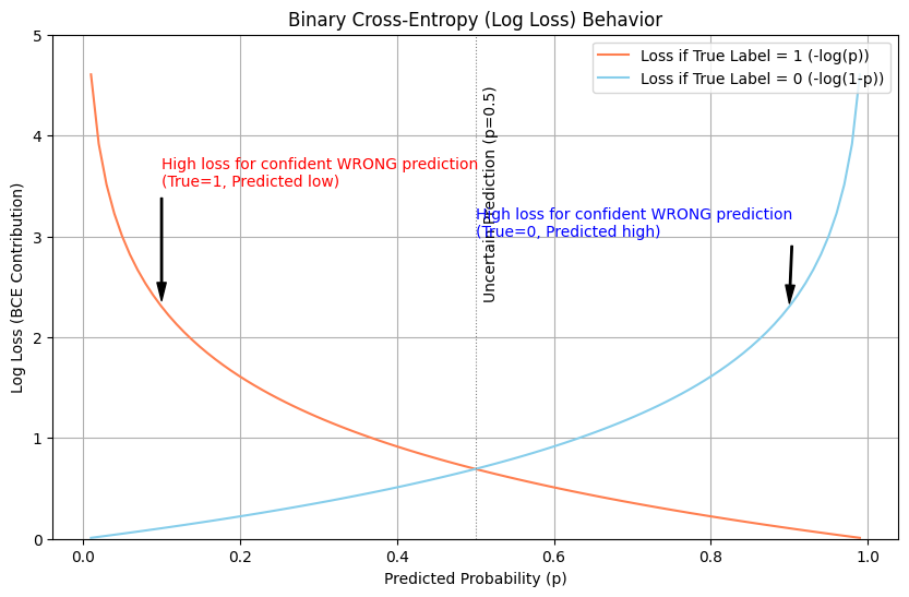
If our model predicts \(\widehat{y}=0.99 \) (very confident and correct), the loss is \(−\log(0.99)≈0.01 \), a very small penalty. But if it predicts \(\widehat{y}=0.01 \) (very confident and wrong), the loss is \(−\log(0.01)≈4.6 \), a huge penalty!
Case 2: The true label is 0 (e.g., “not spam”)
Now the first term, \(y \), is 0, wiping out the first half. We are left with:
$$
\text{Loss} = -\left[ (1-0)\,\log\Bigl(1 – \widehat{y}\Bigr)\right] = – \log\Bigl(1 – \widehat{y}\Bigr)
$$
If our model predicts \( \widehat{y}=0.01 \) (meaning it’s 99% sure it’s not spam, so it’s confident and correct), the loss is \(−\log(1−0.01)=−\log(0.99)≈0.01 \), again a tiny penalty. If it predicts \( \widehat{y}=0.99 \) (confident and dead wrong), the loss is \(−\log(1−0.99)=−\log(0.01)≈4.6 \), another massive penalty.
The use of the logarithm is key. As the predicted probability approaches the wrong answer (e.g., predicting 0 when the answer is 1), the log value plummets towards negative infinity, making the loss skyrocket. This gives the model a very strong “signal” during training to correct its course.
The Grand Inquisitor of Generative AI: BCE in GANs
The role of Binary Cross-Entropy truly shines in the adversarial world of Generative Adversarial Networks (GANs). A GAN is a fascinating AI architecture composed of two dueling neural networks:
- The Generator: Its job is to create fake data (e.g., images of faces, musical notes) that looks indistinguishable from real data.
- The Discriminator: Its job is to act as a detective, looking at an image and deciding if it’s real (from the training dataset) or fake (created by the Generator).
This is a perfect binary classification problem! The Discriminator’s output is a probability—the likelihood that the input it sees is real. And so, its performance is measured using Binary Cross-Entropy.
The training process is a brilliant tug-of-war:
- Training the Discriminator: We show the Discriminator a mix of real images (label = 1) and fake images from the Generator (label = 0). The Discriminator calculates its predictions, and we use BCE to compute its loss. This loss tells us how bad the Discriminator is at telling real from fake. We then use this loss to update the Discriminator’s parameters to make it a better detective.
- Training the Generator: Here’s the genius part. We freeze the Discriminator and have the Generator produce a batch of fake images. These are fed to the Discriminator. The Generator’s goal is to fool the Discriminator into thinking its fakes are real (i.e., to make the Discriminator output a “1”). So, the Generator’s loss is calculated using BCE, but with the labels for its fake images flipped to 1. If the Generator creates an image that the Discriminator confidently calls fake (e.g., a probability of 0.1), the Generator’s loss will be high \((−\log(0.1)≈2.3)\). This high loss signals the Generator to adjust its own parameters to produce more realistic images.
In this dance, BCE serves as the universal language of success and failure, driving both networks to improve. The Discriminator uses BCE to get better at spotting fakes, and the Generator uses the Discriminator’s BCE-based judgment to get better at creating them.
Here is a simplified Python representation:
import numpy as np

def binary_cross_entropy(y_true, y_pred):
  """
  Calculates the Binary Cross-Entropy loss for a single example.
  y_true: The actual label (0 or 1)
  y_pred: The predicted probability of the label being 1
  """
  # Clip predictions to avoid log(0) which is undefined
  y_pred = np.clip(y_pred, 1e-7, 1 - 1e-7)

  term_1 = y_true * np.log(y_pred)
  term_2 = (1 - y_true) * np.log(1 - y_pred)

  return -(term_1 + term_2)

# --- Discriminator's perspective ---
# It sees a real image (true label = 1) and is 95% sure it's real.
loss_real = binary_cross_entropy(y_true=1, y_pred=0.95)
print(f"Discriminator loss for a good 'real' prediction: {loss_real:.4f}") # Low loss

# It sees a fake image (true label = 0) and is 90% sure it's fake (pred=0.1).
loss_fake = binary_cross_entropy(y_true=0, y_pred=0.10)
print(f"Discriminator loss for a good 'fake' prediction: {loss_fake:.4f}") # Low loss

# --- Generator's perspective ---
# The Generator wants its fake image to be classified as real (target label = 1).
# The Discriminator is 90% sure it's fake (pred=0.1).
generator_loss = binary_cross_entropy(y_true=1, y_pred=0.10)
print(f"Generator's loss for a poor fake image: {generator_loss:.4f}") # High loss
A Specialised Tool in the LLM Workshop
Now, what about Large Language Models (LLMs) like ChatGPT or Llama? The core task of an LLM during its initial training is next-token prediction. Given a sequence of text like “The cat sat on the,” the model must predict the next word (or “token”). This is not a binary choice. The model is choosing from a vocabulary of tens of thousands of possible tokens.
This is a multi-class classification problem, and for this, a more general version of cross-entropy is used: Categorical Cross-Entropy. It’s the big brother of BCE, designed to handle situations with more than two possible outcomes.
So, if LLMs don’t use BCE for their primary training, where does it fit in? BCE becomes a vital tool during the fine-tuning and application phases, when we adapt a general-purpose LLM for a specific binary task.
Consider these common applications:
- Sentiment Analysis: We can take a pre-trained LLM and fine-tune it to classify a movie review as “positive” (1) or “negative” (0). We add a new “head” to the model—a final layer that crunches the LLM’s complex text representation into a single probability. This final layer is then trained using Binary Cross-Entropy on a dataset of labeled reviews.
- Fact-Checking: Given a statement, is it “true” (1) or “false” (0)? Again, an LLM can be fine-tuned for this binary task, with BCE as the driving loss function.
- Duplicate Question Detection: On a forum like Stack Overflow, we might want a model to determine if two questions are duplicates of each other (1) or not (0). BCE is the perfect loss function to train this specialized model.
In these cases, the massive, pre-trained LLM acts as a powerful feature extractor, understanding the nuances of the input text. BCE then provides the simple, focused objective needed to steer that understanding toward a specific binary decision.
The Elegant Power of a Simple Question
Binary Cross-Entropy is a testament to the power of finding the right way to ask a question. It doesn’t just ask, “Is the model right or wrong?” It asks a more profound question: “How surprised should we be by the model’s prediction, given what we know to be true?“
By punishing confident but wrong predictions most severely, it forces models to learn not just the answers, but also the subtleties of probability and uncertainty. From simple email filtering to the adversarial ballet of GANs and the specialised applications of LLMs, BCE is the quiet, rigorous teacher that guides our most powerful algorithms toward making better judgments, one coin flip at a time.
Test Your Understanding
To solidify these concepts, reflect on these questions:
- Why is the logarithm function so critical to BCE? What would happen if we simply used the linear difference between the true label and the predicted probability (e.g.,
Loss = y - y_hat)? - The “Clipping” in the Code: In the Python example,
y_predis “clipped” to be within a tiny margin of 0 and 1. Why is this numerically important when implementing BCE? What mathematical problem does it prevent? - BCE in a Multi-Label World: Imagine you’re tagging a blog post. It could be tagged with “Tech,” “AI,” “Startups,” etc. A single post can have multiple tags. Is this a binary classification or multi-class classification problem? Could you use BCE here? (Hint: Think about treating each tag as an independent yes/no decision).
- A Practical Thought Experiment: You’re building a simple AI to approve or deny loan applications. Your model outputs the probability of a person defaulting on the loan. For a specific applicant who, in reality, did not default (label=0), would you, as the bank, prefer your model to have predicted a default probability of 0.6 or 0.9? Which prediction would result in a higher BCE loss, and why is that desirable?
Enjoyed this deep dive? This post is one part of a larger journey into the core concepts of AI. To build a solid foundation and see how all the pieces connect, I recommend exploring the series from the beginning:
- Start with the Core Paradigms Videos:
- Understand the Engine of Learning:
1 thought on “The Art of Judging a Coin Flip: Binary Cross-Entropy in the AI Universe”
Comments are closed.