
Imagine you’re teaching an archery student. They loose an arrow, and it thuds into the target, a little off-center. You wouldn’t just say, “You missed.” To be a good teacher, you need to know how much they missed by. Was it a near-perfect shot, just a hair’s breadth from the bullseye? Or did it land in another post code entirely? The better you can measure the error, the more effectively you can guide your student’s next attempt.
In the world of Artificial Intelligence we face a similar challenge. We build these complex models to make predictions, generate images, or write text. But how do we know if they’re any good? How do we guide them from making nonsensical guesses to producing insightful, accurate, or beautiful outputs? The answer, in many cases, lies in a surprisingly simple yet profoundly powerful mathematical concept: Mean Squared Error (MSE).
At its heart, MSE is a way to measure the “unhappiness” of our model. It quantifies the average of the squares of the errors—that is, the average of the squared differences between what the model predicted and what actually happened. Let’s break this down, piece by piece, to truly understand its elegance and importance.
From a Single Mistake to a Grand Average: The Anatomy of MSE
At its core, Mean Squared Error is a way to quantify the difference between a predicted value and an actual, true value. Let’s build it from the ground up.
Imagine a simple AI model trying to predict tomorrow’s temperature. It predicts 25°C, but the actual temperature turns out to be 27°C.
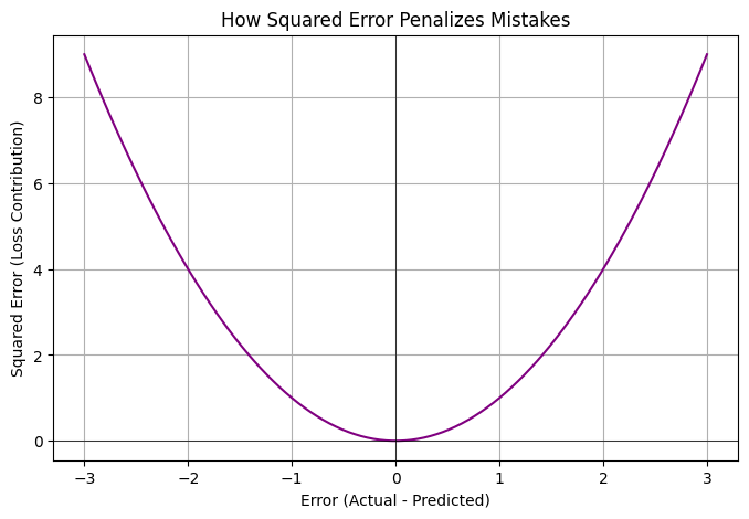
- The Error (or Residual): The most basic measure of our mistake is the difference.\(Error=Actual Value−Predicted Value=27−25=2\). But what if the prediction was 29°C? The error would be \(27−29=−2\). If we just averaged these errors, a +2 and a -2 would cancel out, suggesting our model is perfect when it’s consistently wrong. We need a way to treat all errors as a form of penalty, regardless of their direction.
- The “Squared” Solution: The mathematical equivalent of saying “a miss is a miss” is to square the error.Squared Error for prediction 1=\((2)^2=4\) Squared Error for prediction 2= \((−2)^2=4 \). By squaring, we solve two problems at once. First, all errors become positive. Second, we disproportionately punish larger errors. An error of 2 becomes a penalty of 4, but an error of 10 becomes a much larger penalty of 100. This is often desirable; in many systems, one catastrophic mistake is worse than a dozen minor ones. Think of an AI piloting a drone: a 1-foot error in landing is acceptable; a 100-foot error is a disaster.
- The “Mean” to Rule Them All: A single squared error tells us about one prediction. To judge the model’s overall performance, we need to look at its performance across many predictions. So, we take the average, or “mean,” of all the squared errors. If we have n data points:$$ MSE=\frac{1}{n} \sum_{i=1}^{n}(Actual_i−Predicted_i)^2$$This formula, in its beautiful simplicity, gives us a single number representing our model’s total “unhappiness.” Our goal during training is to make this number as small as possible.
MSE as the Engine of Classical AI: The Art of Finding the Bottom
In traditional machine learning, especially for regression tasks (predicting continuous numbers), MSE isn’t just a report card; it’s the engine of learning itself. Consider the classic task of fitting a line to a set of data points.
Imagine the MSE as a vast, three-dimensional landscape. The two horizontal dimensions represent the possible values for the parameters of our line (its slope and intercept). The vertical dimension represents the MSE for that particular line. Our goal is to find the lowest point in this landscape—the “valley” where the error is minimal.
This is where the magic of gradient descent comes in. By calculating the derivative (the slope) of the MSE function, we can determine the steepest direction at our current location. To find the minimum, we simply take a small step in the opposite direction—downhill. We repeat this process, iteratively adjusting the line’s parameters, and with each step, our line gets a little bit closer to the best possible fit for the data.
The smooth, bowl-like shape of the MSE function (it’s a convex function) is a godsend for this process. It guarantees that there is only one global minimum, so our downhill journey will inevitably lead us to the best possible solution.
Bowl-like shape of the MSE function
Here’s a quick look at this in action with a Python code snippet:
import numpy as np

# Ground truth values (e.g., actual house prices)
y_true = np.array([250000, 300000, 450000, 500000])

# Our model's initial, naive predictions
y_pred = np.array([230000, 330000, 420000, 480000])

# 1. Calculate the errors
errors = y_true - y_pred
# errors -> array([ 20000, -30000,  30000,  20000])

# 2. Square the errors
squared_errors = errors ** 2
# squared_errors -> array([400000000, 900000000, 900000000, 400000000])

# 3. Calculate the mean of the squared errors
mse = np.mean(squared_errors)
# mse -> 650000000.0

print(f"The model's initial Mean Squared Error is: {mse}")
# The learning process (e.g., gradient descent) would now adjust the
# model's internal parameters to make y_pred closer to y_true,
# thus systematically lowering this MSE value.
A New Canvas for an Old Tool: MSE in Generative AI
So, MSE is great for predicting numbers. But how can it possibly help an AI generate a photorealistic image of an astronaut riding a horse, or a hauntingly beautiful piece of music? The answer is that MSE is repurposed from being a direct measure of final quality to a fine-grained tool for learning internal representations and processes.
Autoencoders: Learning to See by Reconstructing
An autoencoder is a type of neural network designed to learn a compressed representation of data. It consists of two parts: an encoder that squishes a high-dimensional input (like an image) into a much smaller, dense vector (the “latent space”), and a decoder that attempts to reconstruct the original image from this compressed information.
The training objective here is simple: minimise the MSE between the pixel values of the original input image and the reconstructed output image. The network isn’t being told what a “cat” or a “tree” is. It’s only being told: “Whatever you do, the end result must look as close to the beginning as possible.” To succeed with the bottleneck in the middle, the network is forced to learn the most essential features of the data—the very essence of what makes an image an image. This learned ability to reconstruct is a foundational step towards generation.
Diffusion Models: Creating Masterpieces by Un-doing Messes
Perhaps the most spectacular use of MSE in modern generative AI is in diffusion models, the powerhouses behind models like DALL-E 2 and Stable Diffusion. Their process is one of the most beautiful ideas in recent AI research:
- The Forward Process (Controlled Destruction): You start with a perfect, clean image. In a series of hundreds of steps, you add a tiny, controlled amount of random noise (think of it as digital static). At the end of this process, the original image is completely obliterated, leaving nothing but pure, random noise.
- The Reverse Process (The Magic of Denoising): This is where the learning happens. A powerful neural network (often a U-Net) is shown a noisy image from the process above. Its task is to predict the exact noise that was added to the image at that step.
How is it trained to do this? By minimising the Mean Squared Error between the noise it predicted and the actual noise that was added.
This seems almost comically simple. The model isn’t trying to predict the final image. It’s just trying, at every stage of corruption, to predict the static. But by becoming exquisitely good at this one, narrow task, the model implicitly learns the entire statistical structure of the training data. It learns what “image-like” patterns look like at every possible level of noise.
To generate a completely new image, you simply start with a fresh patch of random noise and ask the model to perform this reverse process. It predicts the noise in the random patch, subtracts a little bit of it, looks at the result, predicts the remaining noise, subtracts a bit more, and so on. Step by step, it “denoises” its way from pure static to a coherent, complex, and often stunningly beautiful new image. MSE is the humble compass that guides every single one of those thousands of steps.
The Subtle Role of MSE in Large Language Models
What about LLMs like GPT-4? When an LLM generates text, its core task is to predict the next word (or, more accurately, “token”) in a sequence. If the input is “The cat sat on the,” the model needs to predict “mat.” This is fundamentally a classification problem, not a regression problem. The model is choosing the most likely token from a vast vocabulary of tens of thousands of possibilities. For this, a different loss function called Cross-Entropy Loss is far more suitable and is indeed the primary workhorse for training LLMs.
So, does MSE have any role to play? While it’s not the star of the show, it appears in important supporting roles, particularly in the expanding world of multimodal AI.
Imagine you want an LLM to understand not just text, but also gestures. You could have a camera that captures a hand gesture and converts it into a numerical representation (an “embedding”). But this gesture embedding “lives” in a different mathematical space from the LLM’s word embeddings. How do you teach the model that the gesture for “for loop” should mean the same thing as the text “for loop”?
One powerful technique is to use MSE as an alignment loss. You would train a small adapter model to take the gesture embedding and transform it into a new embedding. The goal of this adapter is to minimise the MSE between its output embedding and the pre-existing embedding for the text “for loop” inside the LLM. By forcing these two vector representations to be as close as possible, you are effectively teaching the model a new “language,” bridging the gap between vision and text. In this context, MSE acts as a translator, ensuring that meaning is preserved across different data types.
Questions to Deepen Your Understanding
The true test of understanding is being able to reconstruct and question an idea. Here are some thoughts to ponder:
- The Outlier Problem: MSE heavily penalises large errors. Imagine you’re training a model to predict house prices, but your dataset includes a few multi-billion-dollar castles. How would these outliers affect the training process if you use MSE? Would the model become better or worse for predicting “normal” house prices?
- MSE vs. MAE: An alternative to squaring the error is to take its absolute value (Mean Absolute Error, or MAE). MAE doesn’t penalise large errors as harshly. When might you prefer MAE over MSE, or vice-versa?
- The Nature of Noise: In a diffusion model, the AI is trained to predict noise. When you ask it to generate an image from pure static, where does the “creativity” come from? Why doesn’t it just generate a noisy mess every time?
- A Practical Thought Experiment: Imagine you’re building a simple AI to control a thermostat. Your target is 22°C. The current temperature is 20°C. Your AI can only adjust the temperature by a fixed amount each minute. How could you use the principle of MSE (the squared difference between the current and target temperature) to decide whether to turn the heat up or down? What is the “parameter” you are adjusting in this simple model?
2 thoughts on “The Subtle Art of Being Wrong: Mean Squared Error and its Guiding Hand in AI”
Comments are closed.