Loss Functions in Machine Learning: AI’s Key Critic Explained

Welcome back to All that is under the Sun! In our last blog post in Learning AI Series, we unmasked “Optimization,” the tireless engine that helps AI models strive for their “best selves.” We saw how AI isn’t just born brilliant; it learns and improves through a process of iterative refinement. But that begs a rather important question: How does an AI model actually know if it’s getting better? How does it tell a “good” prediction from a “total facepalm” moment?

Enter the unsung hero of the machine learning world: the Loss Function. Think of it as AI’s brutally honest best friend, its personal trainer who doesn’t pull punches, or its built-in “Ouch Meter!” It’s the critical voice that tells the AI, “Nope, that wasn’t quite it, try again!” but also, “Ooh, much better! You’re getting warmer!”

Today, we’re demystifying loss functions – what they are, why they’re the linchpin of AI training, and crucially, why understanding them is vital whether you’re building an AI from scratch or working with those powerful pre-trained models everyone’s talking about. Fasten your seatbelts; this is where the learning really learns how to learn!

What in the AI World is a Loss Function? The Bare-Bones Intuition

At its core, a loss function (also known as a cost function or error function) is a mathematical way to measure how badly your AI model’s predictions missed the mark compared to the actual, real-world truth. It quantifies the “wrongness” of a prediction into a single numerical score. The higher the score, the worse the model did. The lower the score, the closer it was to the desired outcome. The ultimate goal during training? You guessed it: minimise this loss score.

Imagine you’re learning to play darts 🎯.

• If you hit the bullseye, your “loss” is zero (Woohoo!).
• If you hit the outer ring, your “loss” is a small number (Not bad!).
• If your dart ends up decorating the wall next door… well, that’s a BIG loss (and maybe a call from the neighbors!).

A loss function does exactly this for an AI model. For every prediction it makes, the loss function calculates a penalty. It’s the judge in an AI talent show, and it’s not afraid to give low scores for off-key performances!

This “score” is super important because it creates what data scientists call a loss landscape. Picture a hilly terrain with mountains and valleys. Each point on this terrain represents a particular set of your model’s internal parameters, and the height of that point represents the loss value. The goal of training, as we saw with optimisation, is to find the deepest valley – the point of minimum loss.

Why Should You Lose Sleep Over Loss Functions? (Okay, Maybe Just Pay Close Attention!)

Understanding loss functions isn’t just academic fluff; it’s profoundly practical. It’s like trying to be a chef – you absolutely need to understand how to taste your food and judge its flavor (the “loss”) to improve your cooking.

When Training New Models from Scratch:

If you’re building and training your own AI model, the loss function is your guiding star.

• Directs the Learning: The optimiser (like Gradient Descent, our friendly mountain hiker from last time) literally uses the output of the loss function (and its slope, or gradient) to figure out which direction to tweak the model’s parameters. No loss function, no direction, no learning. It’s like trying to navigate a maze blindfolded and without your hands – pretty useless!
• Defines “Good”: Your choice of loss function inherently defines what your model will prioritize learning. If you choose a loss function that heavily penalizes certain types of errors, your model will work harder to avoid those specific errors. It shapes the very “soul” of your model.
• The Right Tool for the Job: Using an inappropriate loss function is a recipe for disaster. Imagine trying to train a model to classify images of cats and dogs (a classification task) but using a loss function designed for predicting house prices (a regression task). Your model would be utterly confused, like a dog told to meow. It would optimize for something completely irrelevant to its actual goal! (Cue sad AI noises 🤖😭).

When Working with Powerful Pre-trained Models (This is HUGE!):

In today’s AI world, we often use pre-trained models – giants like GPT, BERT, or Stable Diffusion that have been trained on massive datasets by organisations with equally massive computing resources. You might think, “Phew, someone else already picked the loss function, I don’t need to worry!” Wrong! Understanding their original loss function is still critical:

• Understanding Model Behavior & Capabilities: The loss function used to train a pre-trained model tells you what that model was originally optimized for. This is key to understanding its inherent strengths, its potential weaknesses, and even its biases. For example, a model trained with a loss function that prioritizes perplexity in language generation might be great at sounding fluent but not necessarily at being factual.
• Smarter Fine-Tuning: Fine-tuning is the process of taking a pre-trained model and further training it on a smaller, task-specific dataset.
  • Compatibility is Key: Should you use the same loss function as the original training for your fine-tuning? Or a new one? If your fine-tuning task has different nuances of “error” than the original task, you might need to adapt or change the loss function. For instance, if a pre-trained image model was trained to identify general objects, but you’re fine-tuning it to detect tiny, critical defects in manufacturing, your sensitivity to false negatives might be way higher, and your loss function might need to reflect that.
  • Avoiding Conflicting Goals: If you slap on a new loss function during fine-tuning that drastically conflicts with the original training objectives, you might get suboptimal performance or even “catastrophic forgetting,” where the model loses its powerful pre-trained abilities. It’s like taking that highly trained sheepdog we talked about – originally trained to herd sheep with precision (low loss on “herding errors”) – and then trying to fine-tune it to only chase butterflies using a “butterfly chase maximization” score. It might get confused and forget how to herd sheep!
• Interpreting Performance & Debugging: When a pre-trained model isn’t performing as expected on your specific data, understanding its original loss function can provide vital clues. Perhaps your data has characteristics that lead to consistently high loss values for certain types of errors that the model was heavily penalized for, indicating a mismatch or a need for more careful data preprocessing.
• Informed Model Selection: If you have a choice between several pre-trained models for a task, knowing their original training objectives (and thus, their loss functions) can help you choose the one whose inherent “priorities” best align with your specific needs.
• Recognizing “Silent Failures”: Sometimes a model can achieve decent accuracy on a task but still make critical errors that the original loss function wasn’t sensitive enough to, or that your specific application cares more about. Knowing the original loss helps you anticipate these.

In short, whether you’re architecting from the ground up or leveraging the power of giants, the loss function is your window into the model’s “mind” and your lever for guiding its learning.

Meet Some Stars of the Loss Function World (with Visual Python Goodness!)

There are many types of loss functions, each tailored for different kinds of machine learning problems. Let’s meet two of the most common ones:

Mean Squared Error (MSE) – The Regression Workhorse

Primarily used for regression tasks, where you’re trying to predict a continuous numerical value (e.g., house prices, temperature, stock prices). MSE calculates the average of the squares of the differences between the predicted values and the actual values.

$$MSE = \frac{1}{n} * \sum(y_{actual} – y_{predicted})^2$$

The “squared” part is key:

1. It ensures the error is always positive (no negative loss!).
2. It penalizes larger errors much more heavily than smaller ones. Being off by 4 units results in a squared error of 16, while being off by 2 units results in a squared error of 4. So, the model is strongly incentivized to avoid those big misses!

Imagine we have some true values and our model’s predictions.

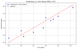
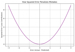
The first plot shows our predictions against the true values. The gray dotted lines represent the individual errors. MSE averages the square of these distances. The second plot clearly shows the parabolic (U-shaped) nature of squared error – small errors contribute a little to the loss, but as the error magnitude increases, the loss contribution shoots up dramatically! This makes the model really want to avoid those big deviations.

Binary Cross-Entropy (BCE) / Log Loss – The Binary Classifier’s Best Friend

Used for binary classification tasks, where the output is a probability that an instance belongs to one of two classes (e.g., spam or not spam, cat or dog, fraudulent transaction or not). The model predicts a probability (e.g., 0.8 for “spam”).

BCE measures how far your predicted probabilities are from the actual class labels (which are typically 0 or 1). It heavily penalizes predictions that are confidently wrong.

• If the true label is 1 (e.g., “spam”) and your model predicts a low probability like 0.1 (meaning it thinks it’s “not spam”), BCE loss will be high.
• If the true label is 1 and your model confidently predicts 0.9, the loss will be low.

Crucially, if the true label is 1 and your model confidently predicts 0.01 (very sure it’s not spam), the loss will be HUGE! This is good – we want to punish confident mistakes. The formula involves logarithms:

$$BCE = (y_{actual} * log (y_{predicted}) + (1 – y_{actual}) * log(1 – y_{predicted})$$

Don’t worry too much about memorising it; the key is its behaviour.

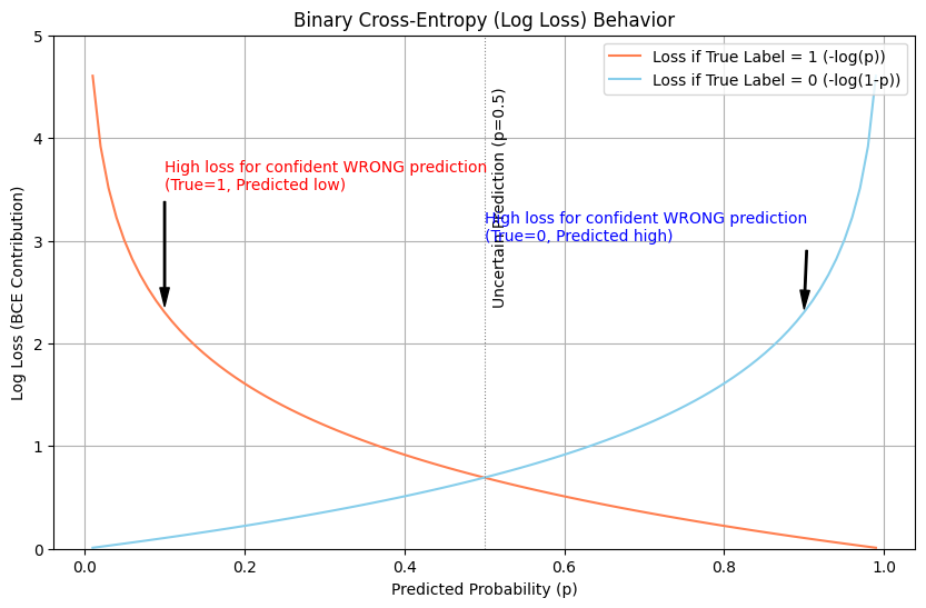
Look at these curves! If the true label is 1 (coral line), the loss approaches infinity as the predicted probability p approaches 0 (confidently wrong). Similarly, if the true label is 0 (skyblue line), the loss skyrockets as p approaches 1. This behaviour powerfully steers the model away from being cocky and incorrect.

These are just two examples. There’s a whole universe of them: Categorical Cross-Entropy for multi-class problems, Huber Loss which is like a mix of MSE and Mean Absolute Error, and many more specialised ones!

Loss Functions & Optimisation: The Perfect Partnership

So, how does our loss function tango with the optimizer we discussed last time?

1. The model makes a prediction.
2. The loss function calculates the error (the “loss score”) for that prediction.
3. This loss score isn’t just a number; it (along with the model’s architecture and parameters) defines that “loss landscape.”
4. The optimizer (like Gradient Descent) then looks at the slope (gradient) of this loss landscape at the current position. The slope tells it which way is “downhill” – the direction that will decrease the loss.
5. The optimizer nudges the model’s parameters in that downhill direction.
6. Repeat millions of times!

The loss function provides the objective, the thing to minimise. The optimiser provides the strategy for how to minimise it. They are two sides of the same learning coin!

A Quick Note on Choosing Your Critic Wisely

While we won’t dive deep into selection strategy today, just remember: the choice of loss function is NOT arbitrary. It fundamentally depends on:

• The type of problem you’re solving: Regression? Binary Classification? Multi-class?
• The specific characteristics of your data and goals: Are some errors more costly than others in your real-world application? You might need a custom loss function (an advanced topic for another day!).

The “Critic” is Your Compass

And there you have it! Loss functions are not just some arcane mathematical detail; they are the very compass that guides an AI model’s learning journey. They are the voice of truth, the measure of progress, and the crucial link between a model’s predictions and the real-world outcomes we care about.

Understanding them empowers you to train better models, make smarter choices when using pre-trained models, and ultimately, to better grasp how AI systems translate complex data into meaningful (and hopefully accurate!) results. It’s like knowing how your car’s GPS actually figures out the best route – it makes you a more confident driver!

In our upcoming posts, we’ll be taking a closer look at Mean Squared Error and Binary Cross-Entropy individually, really getting into their nitty-gritty. You won’t want to miss it!

What are your thoughts? Did you have an “aha!” moment about loss functions today? Or perhaps a pre-trained model experience where understanding the loss was key? Share in the comments below!

Until next time, keep those neurons firing and those loss values dropping! 😉

Stay tuned & stay simplified!